
Large Language Models explained: part 1
What is a transformer? (the "T" in Chat-GPT)

Introduction
After a long break between posts due to grad school and general busyness, here’s my next post. This one is the first in a three part series on large language models. In this series I want to really drill down into the technology behind ChatGPT so people understand how it works.
In this post I explain the architecture behind models like Chat-GPT, the transformer. I explain the background to why transformers are successful and the key to the transformer architecture, the “self attention mechanism”.
The plan is for the second post to go over the other technical details of the GPT series - the architecture isn’t just a transformer! In particular, Chat-GPT and its predecessor Instruct-GPT have a reinforcement learning aspect to their architecture - they are basically a bigger version of GPT-3 that has been fine-tuned with human in the loop reinforcement learning to be good at chat dialogue.
Then for the third post, I will give my overall take on the LLM technology, its limitations, and what I think its future might be. This will be for a general audience.
A fair warning, the first two parts will technical and will requires some understanding of machine learning and maths. Non technical readers, feel free to skip the first two posts accordingly, although the second one will be less technical than this.
Background: Historical Context
Deep Sequence Modelling
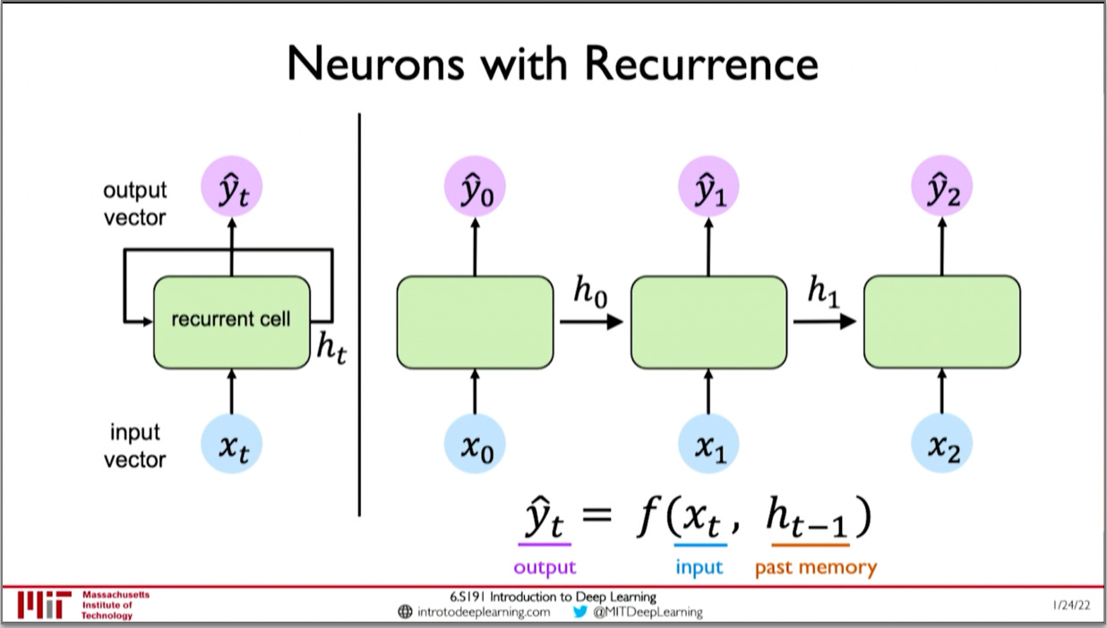
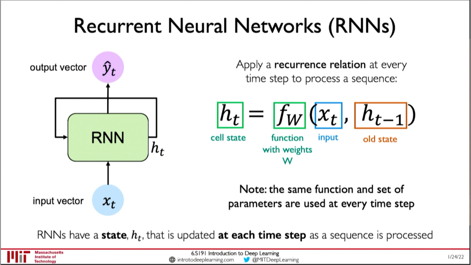
Sequence data is a type of data that has a defined ordering, for example a book, time series data of stocks, and audio recordings are all sequences, of words, prices, and sound respectively. When people started to use machine learning to model sequence data, they used recurrent neural networks, which were created in 1986.1 Recurrent neural networks are feed-forward neural networks that have an internal "state" representation at each time step. Each state is dependant on the state at the previous time step. This gives RNNs the ability to model processes that change over time.
The problem with RNNs
However, RNNs have problems.
Because they are inherently sequential, they cannot be parallelised like other neural networks, making them slower to train and run.
RNN also lose information when modelling long sequences. This is because any given state only directly depends on the previous state. Thus information from states far away is lost
RNN cannot learn bidirectional context, they can only predict a word based on the words that came before it, so they can't look ahead and see how a word fits in a sentence.
Lastly, they fail to train properly if you make them too long. This happens because of the vanishing gradients problem. This occurs when the gradients diverge as they are multiplied back over the long network during back-propagation. This is because the gradient of the state is dependent on the weight matrix and the derivative of the activation function recursively, i.e they are multiplied by them at each back-propagation step. So they are exponentially dependant on these values, and thus may decay or diverge exponentially, which breaks training for a long RNN. Let x_t denote the state at time step t, and x_k denote the state at step k, and W_rec the recurrent weight matrix. Then, we can see from the following equation the matrix product can explode or vanish when it is applied repeatedly during back-propagation if W_rec has a different magnitude than 1.2
LSTM to the rescue
This is where LSTM networks come in.
LSTM networks are a form of RNN which were created to solve the vanishing gradient problem RNNs suffer from. They are a complicated architecture, but essentially they solve the vanishing/exploding gradient problem by changing the gradient update step so that instead of being multiplied by a certain factor repeatedly, a factor is added. So the update operation is changed from multiplication to addition. This means the gradient can no longer vanish and is less likely to explode (although it still can in some situations). This allows memory to be retained for longer sequences. While RNN explode / vanish after ~10 timesteps, LSTMs can learn sequences of up to 1000 time steps.3
However, LSTMs still have a lot of the same problems RNNs do.
Because of the inherently sequential nature they can’t be trained in parallel by a GPU.
They are slow to run as well and can only process data sequentially.
Furthermore LSTMs learn left-to-right context and right-to-left context separately, whereas in reality they are not independent.
So for a while, language models were sort of stuck. Sequential models like RNN and LSTM are inherently limited in terms of how efficient they can be: the deep learning revolution came about as a result of having methods that were able to harness the computation coming from the increasing development of GPUs (graphics processing units). These were developing at an ever increasing pace because people were using them to do wholesome activities like mining bitcoin and playing anime wife simulator at max settings. How did GPUs speed up neural networks? A brief foray into the basics of parallel computing is necessary.
If you have a task that can be broken up into many small subtasks that can be solved at the same time, and then put back together to give your overall solution, computer scientists say your problem is “parallelisable”. Certain problems, are considered “embarrassingly parallel”, because the speedup factor from this is very large, as the problem can be easily split into subtasks, and the subtasks don’t have to share information. GPUs are computer chips designed to do certain types of operations very quickly in parallel, which allows them to compute certain mathematical operations (like matrix multiplication) very efficiently. Computer graphics uses many of these operations to compute lighting and rendering etc, so as I said above, this is why GPUs were originally developed, people wanted games with better graphics. But the same kind of operations also occur in machine learning a lot. So the basic problem with LSTM and RNN is that we have these great big awesome powerful computer chips (GPUs) but because these architectures are not parallelisable (they are inherently sequential), we can’t get the full speedup that we can apply to other neural networks. That’s where the transformer comes in. The essential factor making the transformer highly successful is that it solves all of the problems with RNN, it is parallel (allows for bigger and faster models), it learns bidirectional context, and it doesn’t forget context as two words get further away in the sequence. It does this with two spicy mechanisms called self attention and positional encoding.
Transformers: Attention is all you need
Transformers are a neural network architecture introduced in 2017 by a team at Google Brain.4 Transformers are the “T” in Chat-GPT and other GPT models. They learn a mechanism called "attention" which allows them to learn to pay attention to different parts of the input sequence.
Critically, this new mechanism of attention allows them to learn relationships in a sequence in parallel. In RNN, positional information is encoded in a the sequential nature (i.e the state at N is related to the state at N+1 because it comes before it) whereas in the transformer, positional encoding is used to make sure tokens have information about where they are in the sequence without having to do sequential processing like in the RNN. Or as they say in the paper, “Since our model contains no recurrence and no convolution, in order for the model to make use of the order of the sequence, we must inject some information about the relative or absolute position of the token in the sequence”.
This makes them faster in two ways.
While RNNs pay a O(N) penalty for processing sequentially, transformers parallelise naively in O(1)
RNNs also pay a O(N) cost to correlate words N away in a sentence, while Transformers can learn correlations between far away data points with constant O(1) cost.
They can also learn bidirectional context without learning "left" and "right" context seperately, meaning they can solve problems of the form "The glass of water is **** and it is sitting on the table.", i.e placing a word in a sentence.

In this way, Transformers solved the problems of efficiency and scalability that RNNs had, and were able to leverage increases in compute and data to reach state of the art on many different language tasks.
The key to understanding transformers: attention mechanism
Attention allows the network to focus on the most important parts of the input. Intuitively, attention works like search & retrieval.
Identify which parts of the input to attend at
Extract the features that correspond to these parts.
The attention mechanism does this with three variables: query, key, and value. Continuing with the search analogy, you can think of these variables in the following way:
The queries are the term you are "searching" for
The keys are the possible "matches" in the data set
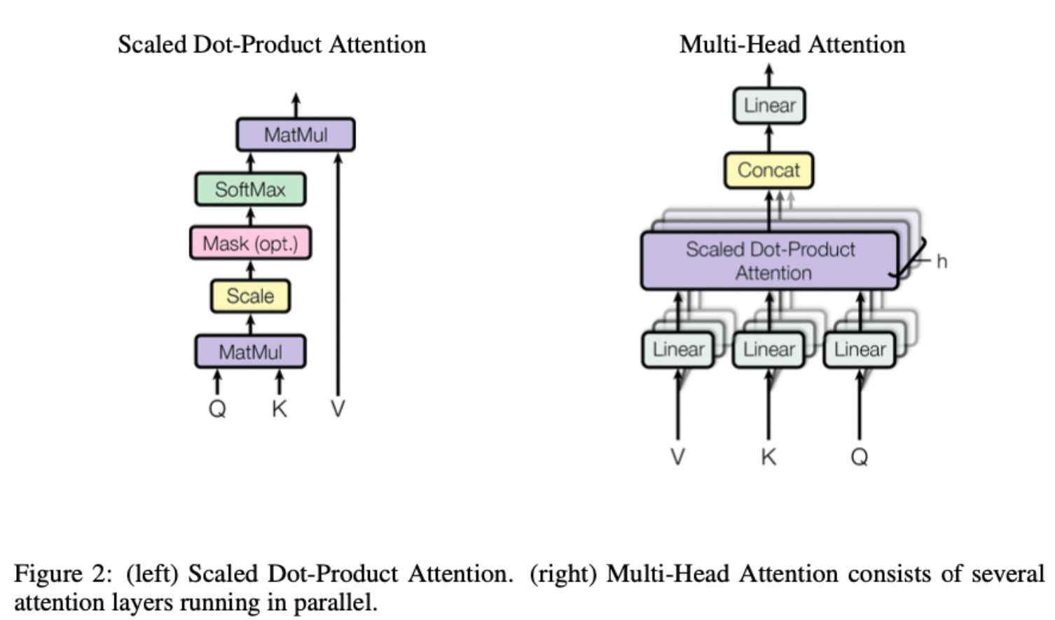
You calculate the correlation / "compatibility" of the queries and keys by creating an attention mask:
Let me explain this equation a little:
Softmax squashes the output so that it all sums to 1.0 (squishing it into probablity space, where likelihoods must add to 1.)
Q and K are matrices made up of the individual query and key vectors.
Thus the matrix multiplication QK^{T} is equivalent to taking the dot product of each query - key vector combination
The dot product q dot k gives us a measure of the similarity of query vector q with key vector k
d_k is the dimension of the key input (length of the keys). Scaling by this stops the dot product from exploding which would break softmax with vanishing gradients
In summary, what we are doing is calculating the similarity of each query with every key, and then doing some scaling to make it easy to work with. This gives us an attention mask.
You can conceptualise the "attention mask" just as you would conceptualise a mask on an image - high for pixels of interest (high similarity of query and key), low for irrelevant pixels (low similarity of query and key).
You then multiply the attention mask by the value matrix (the input values) to extract the part of the input you are paying "attention" to.

And that’s all attention is! It’s a bit of a complicated process, but once you get it, it seems simple. Maybe read this section a few times to let it sink in. I will also run through a numerical example. Again, if you are non technical, you can skip this part.
Self attention example
Say we have the following example for keys and values
And we have the following query matrix that consists of only a single query: (i.e a 1xn matrix)
We get the following result:
The query matches with the second key, so we get a 1.0 weighting on the second entry of the attention mask. Then, we multiply the attention mask by the value vector, extracting the 12.0 feature in the second row.
Let's try two query vectors this time. We still pass them as a matrix.
First we take the query vector
Equally matches the 3rd and 4th keys so we get an attention mask for the first part of
Likewise the second query vector equally matches the first and second keys so we get the following overall attention mask
This gives us the following attention
We can see the extracted features are the average of the 3rd and 4th key-values for the first query and the average of the 1st and 2nd key-values for the second query.
Attention in practice: “the ball is red”
OK, so that is how you calculate the attention of a given key, query, and value matrix. Now I will explain how this would work in an actual textual example.
Take the following string: “The ball is red”.
How do we convert this into the Q,K,V matrices? Well the Query, Key and Value matrices are generated by transforming an input feature matrix, X. The transformations the attention head performs to generate Q,K,V are made by three learned weight matrices, W_{Q}, W_{K}, W_{V}. So the model learns to calculate an accurate attention mechanism for a given feature input by training the weight matrices that generate our Q,K,V.
We could just as easily write the expression for attention as a function of the input feature matrix, and the three weight matrices.
Now let’s go back to the transformer. We’re not done yet, we need to convert the string into a series of vectors to make our Q,K,V. First we must give each word a word2vec embedding and positional information. The word2vec embedding is a way of representing words in a geometric space where similar words like "happy" and "glad" are closer together, and it is learned by running a neural network on a large textual dataset. We have to encode words as vectors because neural networks can't handle strings as input. As for the positional encoding, I described it above, it is essentially a way of encoding spatial information in the word vector. We then have the following sequence (Where E_{The} is the embedding of "The").
When this sequence X is passed into the attention head, it is multiplied with the learned weight matrices to generate the query, key and value matrices, which store the query key and value vectors for every word in the sequence in each row.
Now we pass the Q,K matrices into the attention mask function
This produces a normalised vector for each word in the sequence, where the ith entry in the jth vector is the "similarity" or attention mask coefficient telling us how much attention the jth word pays to the ith word. For our example above that would look like this
Then, we finally multiply this by the "value" vector to extract the final attention result for our feature input. A vector that represents the "attention" for each word in the sequence, where the ith entry is a product of the mask vector for the ith word with the values (which is the entry embedding transformed by the learned weight matrix W_{v}.)
Attention heads, multi-head attention
This process of calculating an attention mask overall represents a neural network called a “attention head” in the transformer model. Here the initial linear layer is our weight matrices W_V, W_K, W_Q. However in the paper many attention heads are trained and run in parallel, to learn to pay attention to several things at once.
More technically, instead of computing a single attention head with d dimensional k,q,v, they compute h smaller attention heads of dimension d/h. This way the model can learn to pay attention to a combination of things in the input. (In the paper, they say "Multi-head attention allows the model to jointly attend to information from different representation subspaces at different positions.")
Where h_n is the output of the nth attention head, defined as above by
Transformers for Translation - The "Attention is All You Need" Network Architecture
Now to put it all together, here is the original transformer architecture, taken from the paper "Attention is all you need" that introduced the transformer. Don’t worry if this seems super complicated, you don’t need to understand this diagram in full as the specifics of this architecture are related to the task the paper was addressing, language translation. I will go through and explain how this works using the concepts we have already covered, and this will give you an idea of how models like GPT use transformers to do natural language processing.
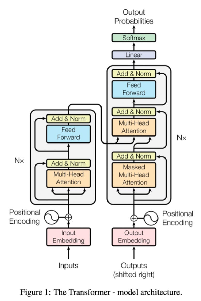
Pass an English sentence to the input embedding.
Input embedding converts each word into to word vector using a pre-trained embedding like word2vec so the network can process it.
With a word embedding, words with a similar "meaning" are embedded close to each-other in a high dimensional vector space (usually around 64 dimensions)
Each word embedding is then given positional encoding. This is a efficient way to store spatial context without having to do the recurrence operation like in the RNN and allows us to compute in parallel.
After word embedding and positional encoding, word embeddings will be closer to each other in the embedding space based on the similarity of their meaning and how close they are to each-other in the sentence
The word embeddings enter the encoder block, where they are input into the multi-head attention block
Each attention head in the multi-head attention block uses learned weight matrices W_{Q},W_{K},W_{V} to transform the input word sequence embedding into a set of query, key and value vectors that form Q,K,V matrices
The query and key matrices are used to calculate a "attention mask", a measure of similarity between each query and key combination, i.e a measure of similarity between every different word
For example: the first entry in the attention mask of the first word embedding would be the similarity of the first word embedding with itself, the second entry would be the similarity of the first word with the second word, etc.
This attention mask is scaled so that the self similarity of an entry with itself doesn't blow out the metric. It is then passed through the softmax function to normalize the distribution
This attention mask is then used to extract an "attention value" for each word. For a given word this will be a weighted sum of each other word embedding, weighted by the attention mask between the given word and each other word.
Here A_{i} is extracted attention value, M_{i,j} is mask between i and j, V_{j} is value corresponding to embedding vector of j (different than the embedding vector itself as it is multiplied by W_{V}).
The result of these individual attention values is combined by the feed forward net to give a single attention vector for each word
The attention vectors are passed into the decoder with the previously generated French word to predict the next French word
The transformer translates a sentence from English to French by maximising the similarity of the attention structure of the inputted English sentence to the generated French sentence.
And that’s how transformers work!
Pat yourself on the back if you made it this far, because this is some heavy stuff. But now that we have this background out of the way, you will understand when I dive into explaining the GPT models and Chat-GPT in the next part of the series. Thanks for reading!
David E. Rumelhart, Geoffrey E. Hinton, and Ronald J. Williams. Learning
representations by back-propagating errors. Nature, 323:533–536, 1986.
Razvan Pascanu, Tomas Mikolov, and Yoshua Bengio. On the difficulty of
training recurrent neural networks. In ICML, 2013.
Ralf C. Staudemeyer and Eric Rothstein Morris. Understanding lstm - a
tutorial into long short-term memory recurrent neural networks. ArXiv,
abs/1909.09586, 2019.
Ashish Vaswani, Noam Shazeer, Niki Parmar, Jakob Uszkoreit, Llion Jones,
Aidan N. Gomez, Lukasz Kaiser, and Illia Polosukhin. Attention is all you
need, 2017.